2 Neoclassical-mainstream consumer choice theory
As explained in the previous chapter, demand curve represents a crucial element of equilibrium and neoclassical theory. What lies behind this famous negative demand curve is neoclassical consumer theory. Neoclassical consumer choice theory has for ambition to explain consumers’ decision, that is to say, the choices consumers make between consuming one good or another. Consumer theory, along with production theory (see following chapter), constitutes an important branch of microeconomics.
Note that this chapter is overall a summary of consumer theory as presented in classical and famous micreconomics textbook. I here especially used Acemoglu, Laibson, and List (2017) and Pindyck and Rubinfeld (2013).
2.1 The three assumptions
Consumer theory makes important assumptions, which are the foundation of the theory:
Completeness:
consumers have complete knowledge about the goods and services they can potentially consume, they have clear preferences about these goods and services and can rank all of them (like a descending list where we would have the most preferred goods and services at the top and utility associated with goods and services would decrease as we go down in the list)
Transitivity:
Preferences regarding goods and services are transitive. That means that if a consumer prefers A to B and B to C, A is better than C.
More is better than less
(non satiety assumption): Goods and services are always desirable. For example, if someone gives you one apple, then two, then three, then twenty, and then one thousands, you would always accept those apples, because you are still better off even if one gives you too many apples.
2.2 Utility function, marginal utility
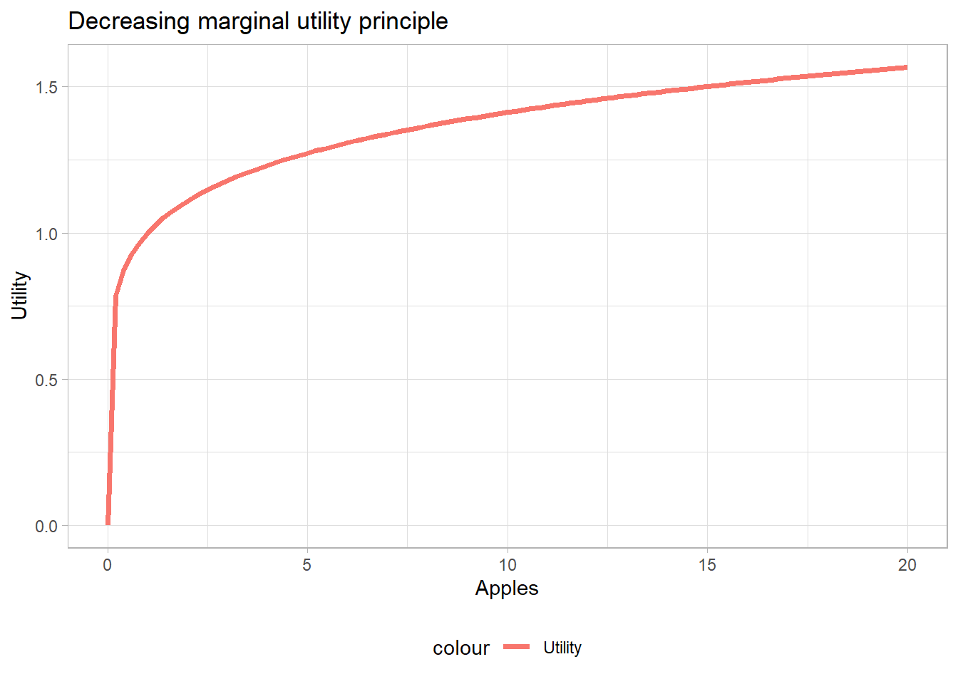
Consumer theory then illustrates any choice between two goods with the help of the famous indifference curves , which show the relation between the demand for one good against the demand for another good (for example food and clothes, cars and bikes…). Indifference curves are based on utility functions whose really important property and assumption is the decreasing marginal utility principle. Decreasing marginal utility means that for every one additional unit of a given good a consumer get, the utility for this consumer increases less than the previous additional unit. Let’s say, for instance, that you don’t have food at the moment and you are hungry: if i give you one apple, you will be a lot better off and your utility will increase a lot when I give you this one apple. Then, if I give you another apple, your utility will still increase, but by less than when I gave you the first apple. Finally, after I give you an additional apple for the fifteenth time, your additional utility will still be positive, but by far more less than when I gave you the first apple.
Decreasing marginal utility is an important assumption which explains the shape of the indifference curves. The latter, if the two goods are substitutes (but not perfect substitute) and not perfect complements, are convex-shaped. If, for instance, we consider an indifference curve for the choice between units of apples and bikes, the line of the indifference curve represents all the possible combination of the two goods which give the same utility for the consumer.
2.2.1 Indifference curve
Indifference curves are based on utility functions. An utility function can be for example:
\[U(x,y)=x^20.18y\]
With x and y two different goods, apples and watches for example. To get the indifference curve function, we fix utility U at any positive value, and rearrange the function above to get y as a function of x and U:
\[U = x^20.18y\]
\[y = \frac{U}{0.18x^2}\]
Yacas vector:
[1] y == U/(0.18 * x^2)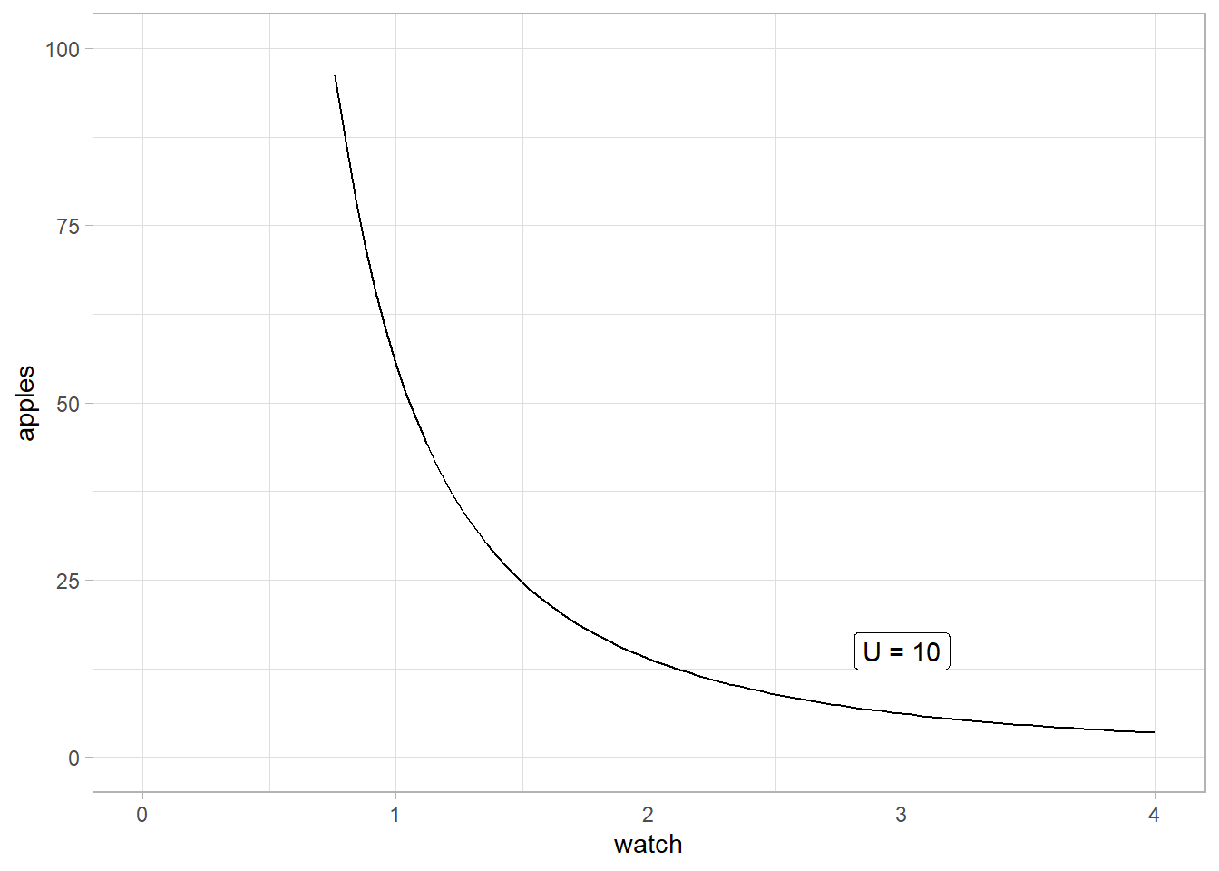
2.3 Budget constraint
In the indifference curve graph above, the consumer can choose any combination of apples and watches on the line, and those combinations would bring the same utility U = 10. However, one important element was not taken into account yet. This element is the fact that consumers are limited in their consumption decisions by their income. Neoclassical theory calls this budget constraint. For instance, let’s say that our consumer has an income of 600 francs. The price of one apple is 4 francs (one bag of apples to be more realistic) whereas the price of a watch is 200 francs. The budget constraint can be written as:
\[ \begin{aligned} Income = P_{apple}*Q_{apple} + P_{watch}*Q_{watch} \\ 600 = 4apple + 200watch \end{aligned} \]
To include this budget constraint into the previous graph, we have to rearrange this equation to have the quantity of apples as a function of the quantity of books:
\[ \begin{aligned} 600 = 4apple + 200watch \\ 4apple = 600 - 200watch \\ apple = 600/4 - 200/4watch \\ apple = 150 - 50watch \end{aligned} \]
More generally, the budget function can also be written as
\[ Q_1 = \frac{Income}{P_1} - \frac{P_2}{P_1}Q_2 \]
Show the code
budget <- function(x) 150 - 50*xNow we can plot both the indifference curves and the budget constraint:
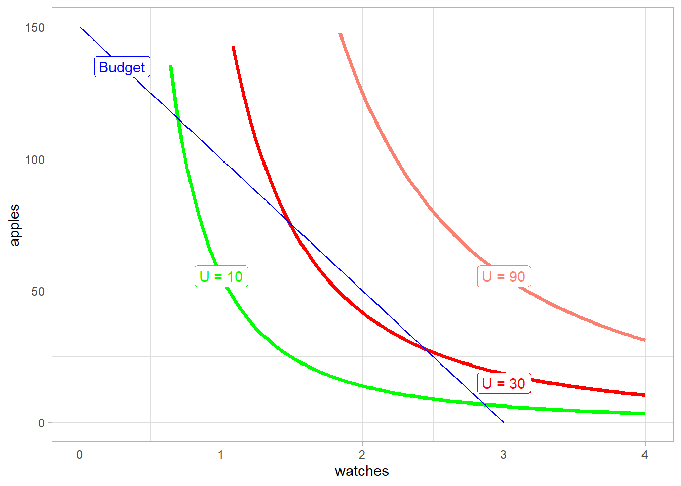
The budget line represents all the combination of apples and watches that the consumer can afford with his income. This implies that is final choice has to be on this line. The consumer cannot afford to be on the U = 90 indifference curve because its income is not large enough. Also, he will not choose any point on U = 10 because the latter’s majority of point are on the left of the budget line (the assumption of more is better than less would not be respected if the consumer for instance chooses 1 watch and 50 apples, because he can afford more of the two goods).
So what will be the consumer’s final choice? He will choose the point at which the budget constraint line is tangent to one of his indifference curve.
Mathematically, this means that the quantity of apples and watches the consumer will choose is the point at which the slope of the budget line \(\frac{P_{watch}}{P_{apples}}\) is equal to the slope of the indifference curve, which microeconomics call the marginal rate of substitution. Marginal rate of substitution shows how much of a good (here apples) the consumer can give up in exchange of one unit of the other good (here a watch). Using algebra, we can find the slope of the budget line and of the indifference curve by computing their derivatives.
\[ \begin{aligned} apple = 150 - 50watch \\ \frac{\partial{apple}}{\partial{watch}} = -50 \\ \end{aligned} \]
Note that finding the marginal rate of substitution is a bit trickier than for the budget line. To find the MRS, we have to compute the derivative with respect to the first good (x which are apples here) and then for the second one (y the watches). Then, the MRS is the ratio between the two marginal utilities
\(\frac{\frac{\partial{U}}{\partial{x}}}{\frac{\partial{U}}{\partial{y}}}\)
\[ \begin{aligned} U = x^20.18y \\ \frac{\partial{U}}{\partial{x}} = 0.36xy \\ \frac{\partial{U}}{\partial{y}} = 0.18x^2 \end{aligned} \]
Thus
\[MRS = \frac{0.36xy}{0.18x^2} = 2\frac{y}{x}\]
Here is how to compute this in R
Then, we set the marginal rate of substitution equal to the slope of the budget line:
\[ \begin{aligned} 2\frac{y}{x} = 50 \\ y = 25x \end{aligned} \]
We can then substitute y with 25x in the budget equation
\[ \begin{aligned} y = 150 - 50x \\ 25x = 150 -50x \\ x = 150/75 = 2 \\ x = 2 \end{aligned} \]
The optimal solution for x (quantity of watch) is thus 2, the consumer will choose 2 watches. Now that know the quantity of watches, we can obtain the quantity of apples as well as how much utility this combination of apples and watches will bring to the consumer.
To get the number of apples, we simply replace x by 6 in the budget constraint equation \(y = 150-50 \times 2 = 50\), \(U = 2^2 \times 50 \times 0.18 = 36\)
R can check the results
Show the code
price_x = 200
price_y = 4
Solve(paste(Simplify(mu_x / mu_y), "==", price_x, "/", price_y), y)
Yacas vector:
[1] y == -(-9 * x/0.36)Show the code
optimal_x <- uniroot(function(x) budget(x) - marginal_utility(x), c(0, 100))$root
optimal_y <- budget(optimal_x)
optimal_u <- utility_u(optimal_x, optimal_y)


optimal_x
[1] 2Show the code
optimal_y[1] 50Show the code
optimal_u[1] 36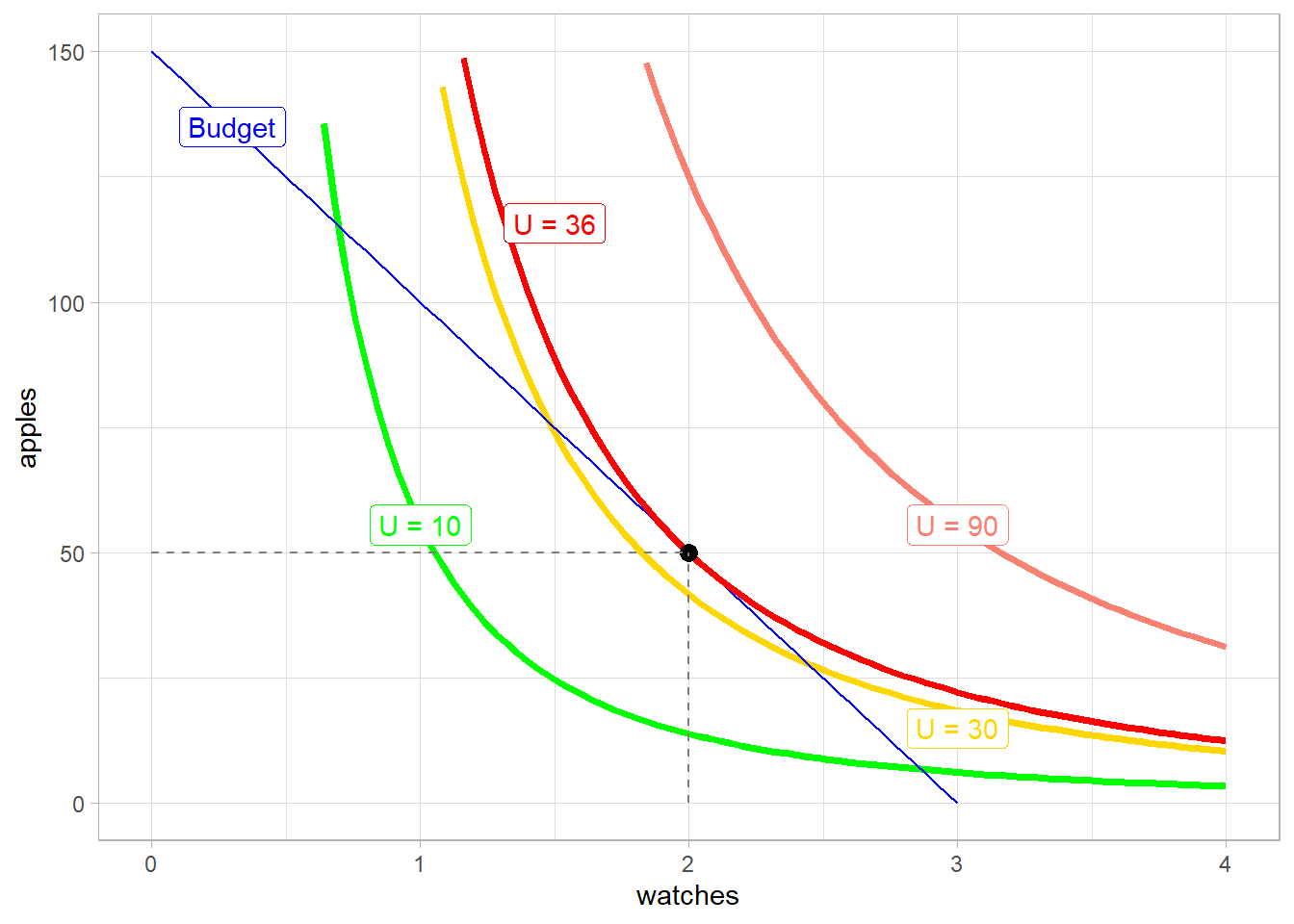
2.4 Deriving the downward slopping demand curve from indifference curve and budget constrain
The final step to grasp why micro theory draws downwards slopping demand curve is to see how a change in relative prices \(\frac{P_2}{P_1}\) changes the consumer’s optimal choice for a good (the equilibrium point in the last graph). In our example, the optimal quantity choice of watch for the consumer was 2 (2 watches costing 200 francs each). What happends in the graph above if the price of watch increases?
The budget constraint will change. Initially we have
\(apple = 150 - 50watch\)
And now, the price of watch increases up to 400, income is unchanged (Income = 600) as well as the price of apples (4):
\[ \begin{aligned} 600 = 4apple + 400watch \\ 4apple = 600-400watch \\ apple = 150 - 100watch \end{aligned} \]
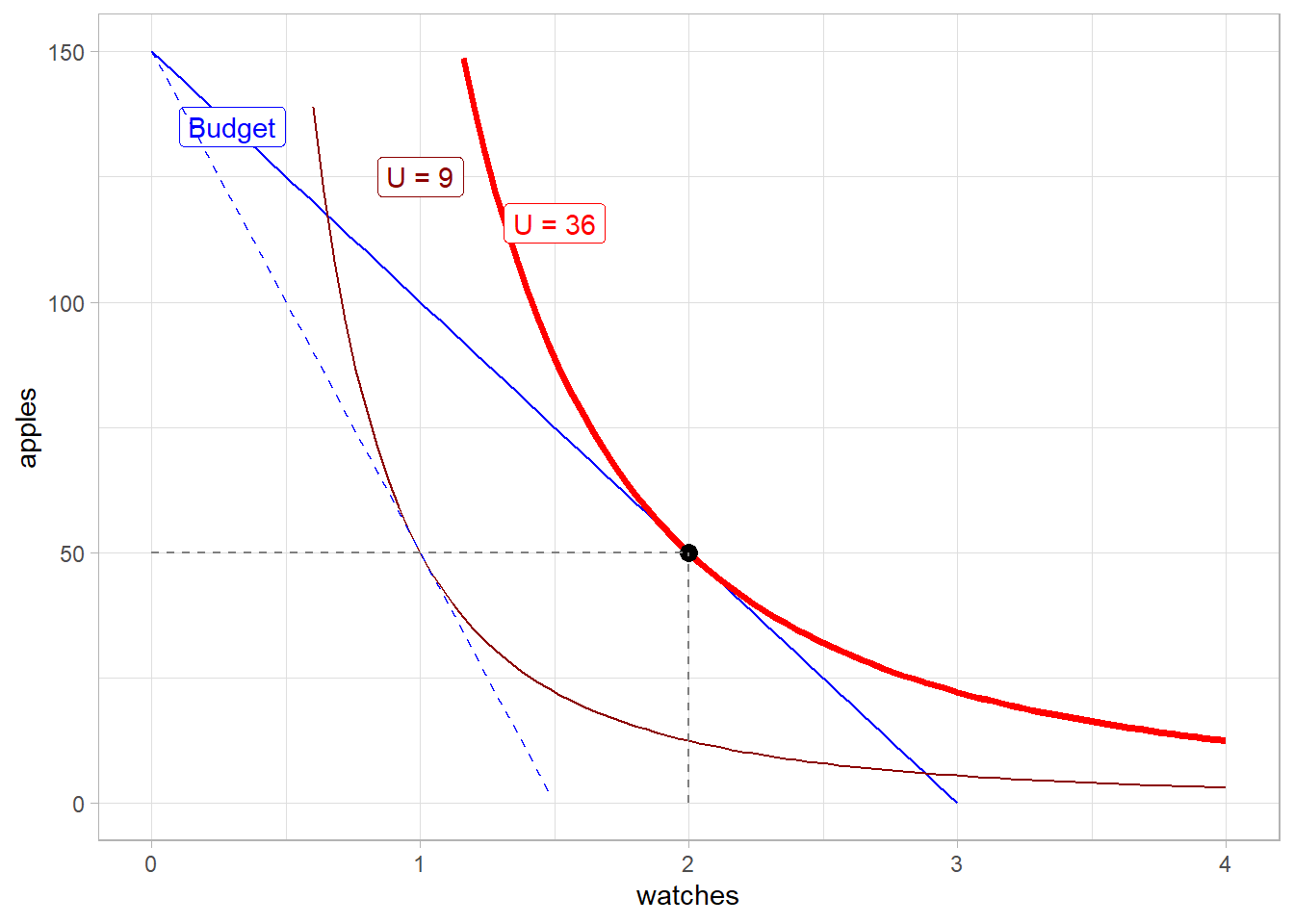
At the new equilibrium level, utility has decreased to 9, apple consumption remains unchanged and the quantity of watches has decreased to one. Note that there are two important mechanisms behind the graph above:
Income effect Income effect relates to how the demand for a good change when income changes. If the demand increases when income increases, micro talks about positive income effect (and conversely negative income effect). In our example, the consumer’s income has not changed (600 francs), but the real income has decreased, because the price of one the good has increased. The consumer has thus a lower (real) income, which led to a decrease in the quantity demanded for the good whose price increased.
Substitution effect Substitution effect refers to how the demand for a good change when the relative price of the good changes.
Income and substitution effects depend on the type of the good. There are indeed different types of goods, depending on how demand changes when price changes:
Normal good
A good is normal when demand increases when its price decreases vice and versa
Inferior good
A good is inferior when the demand decreases as income increases or the price increases
Giffen good
A Giffen good refers to goods whose demand increases when price increases. The logic behind this are the goods which are very essential to every day living (for example staple food): an increase in the price of very essential food can lead to the consumer’s decision of reducing the consumption of other goods to still afford consuming the essential good.
This is how microeconomics derive the demand curve. We will see below that the supply curve is also derived with the same logic, the steps being almost the same as we saw here, but by replacing the utility function with a production function and replacing the two goods by capital and labour, which are the factors of production of any firm.