Show the code
# how to write the leontief production function in R
leontief <- function(l, k, a0, a1) (min(c(l/a0, k/a1)))What follows is extensively based on the second chapter of Heterodox Macroeconomics: Models of of Demand, Distribution and Growth (2019) by Robert A. Blecker and Mark Setterfield
The classical-marxian model, named after Smith, Ricardo (who are considered as classics) and marx and based on their important work, comes with these specific assumptions:
The latter, \(u = \frac{Y}{Y_{K}}\), is ratio of the actual output (GDP) divided by the full capacity output \(Y_K\), which is the level if output if all capital in the economy was used at its full capacity (no unused machines, raw materials…). If this ratio is equal to one, that means that the economy is at full capacity, the actual output is equal to its capacity level. If the ratio is for example 0.5, that means that actual output is half its level if all capital was fully used. But why does this model make such an assumption? This assumption stands in sharp contrast with the (neo)kaleckian model which typically reverses this assumption stating that capacity rate \(u\) is an important adjusting variable.
Before explaining the reason behind this assumption, it is necessary to understand the classical-marxian conception of the production process (how inputs, capital and labor, are combined to produce either goods or services), which rests on the Leontieff production function. The latter can be written as
\[ Y = min(\frac{N}{a_0}, \frac{K}{a_1}) \tag{5.1}\]
With N and K respectively labor and capital, \(a_0 = L/Y\) the labour-output ratio (the quantity of labour required to produce one unit of ouput) and \(a_1 = K/Y\) the quantity of capital required to produce one unit of output (capital-output ratio).
\(\frac{N}{a_0}\) is the maximum output that can be produced with available labour resources while \(\frac{K}{a_1}\) represents maximum output when all capital resources are used.
For instance, if three units of labor are required to produce one unit of output and one unit of capital is required to produce one unit of output, what will be produced if we have N = 9 and K = 4 ?
In our example, \(a_0 = 3/1\) (three units of labor required to produce Y = 1) and \(a_1 = 1\) (one unit of capital to produce one unit). We compute \(N/a_0 = 9/3\) and \(K/a_1 = 4/1\). Since the former \(9/3 = 3\) is bigger than \(4\), all 9 units of labor will be used to produce 3 units of output. Note that at Y = 3, one unit of capital will be leftover and be unused. In this example, output is “labor-constrained” because it is the amount of labor which is fully used and capital which is not. Output at full employment is \(Y_N = N/a_0\).
Considering labor as the constraint is what the (neo)kaleckian model does, while the classical-marxian model considers that capital is the binding constraint on potential output. In the classical-marxian model, all capital is used and thus output is output at full capital utilization \(Y_K = K/a_1\).
While both classical-marxian and (neo)kaleckian models use Leontief production function (and are here different from neoclassical models which use cobb-douglas production function), they differ by what they consider as the constraining factor on output: labor for (neo)kaleckian model \(Y_N\), capital for classical-marxian model \(Y_k\).
Thus, considering that capital is the constraint implies the possibility to consider that the economy can reach a full capacity utilization \(u = Y/Y_k\), this is what the classical-marxian model does thus why \(u\) is considered constant at full capacity \(u = 1\).
There is no technological change in the classical-marxian model. However, the effects of exogenous technological change can still be analyzed.
The main equation is derived from the income approach to national income, which is an accounting identity showing that national income is the sum of all income sources in the economy. The model makes here other assumptions: no government, closed economy, only workers and capitalists, only one good produced, which are nessecary to write:
\[ PY = WL + rPK \tag{5.2}\]
Which is the national income identity after those assumptions, with \(P\) the price, \(Y\) the output, \(W\) the nominal wage rate, \(L\) the amount of labor employed, \(r\) the profit rate and \(K\) the real stock of capital.
From this equation above is derived one the main equation of the model, the inverse wage-profit relationship:
\[ w = \frac{1}{a_0}-\frac{a_1}{a_0}r \tag{5.3}\]
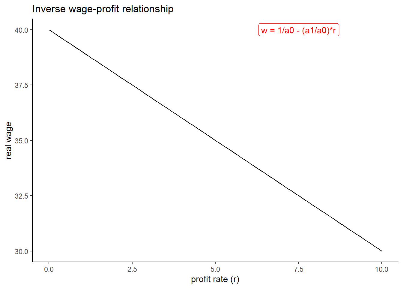
This equation also implies an inverse relationship between consumption and growth
\[ c = \frac{1}{a_0}-\frac{a_1}{a_0}g \tag{5.4}\]
With \(c\) consumption of both workers and capitalist and \(g\) the rate of capital accumulation \(g = \Delta{K}/K = I/K\)
These two relationships and hence trade-off between wage and profit, and consumption and growth are the implications of the two main assumptions explained above: constant rate of capacity utilization and given constant technology. Technological change or rise in \(u\) can improve the wage-profit trade-off and thus make both profits and wage rate rise (same for consumption-growth trade-off). Graphically, the slope of the curve above would either shift upward or one of the intercept increase.
The model makes here another important assumption: all saving is done by the capitalist class. All savings come out from of the profits received by the capitalists. Another important feature is the fact that the classics and Marx did not distinguish between savings and investment (“the purchase of newly produced capital goods, such as machinery, equipment or structures”(p.63)). In C-M terminology, “accumulation” means the mechanistic flow between savings, investment and thus growth. This leads to the “accumulation function”:
\[ g \equiv I/K \equiv S/K = s_r(r-r_{min}) \tag{5.5}\]
\(g \equiv I/K \equiv S/K\) (growth \(g\) is equal to the investment rate \(I/K\) which is the same as saving rate \(S/K\)) comes from this non-distinction between saving and investment. \(s_r\) is the proportion capitalists save out of their profits \(r\). This equation means that growth can increase only with an increase in the saving rate of the capitalists.
The basic model is thus based on the three main equations
\[ w = \frac{1}{a_0}-\frac{a_1}{a_0}r \]
\[ c = \frac{1}{a_0}-\frac{a_1}{a_0}g \]
\[ g \equiv I/K \equiv S/K = s_r(r-r_{min}) \]
However, the model is not “closed” in the sense that all the main variables (w, r, s_r, g) are endogenous (they all are a function of one another). The model needs thus to be “closed” by adding an exogenous variable. Since the classics and Marx did not give a precise and consistent closure (exogenous variable), the textbook gives four “alternative closures” which come from different interpretation the classics and Marx.
Which represents an ordinary standard of living for a working-class family. This should not be confounded with the infamous “iron law” of wages (that wages will always tend to go to the subsistence level, this was made popular by Ferdinand Lassalle and Malthus but has nothing to do with Marx and the classics). This exogenous wage rate \(\bar{w}\) is given, but socially and historically determined and varies across countries and time. This is not a natural/physical minium subsistence wage.
This assumes that wages are determined through a bargaining process in which workers can bargain with capitalists to get wages such as a given wage share of national income is achieved. Note that the wage share can be written as \(\psi = wa_0 = w*L/Y\) and the profit share \(\pi = ra_1=rK/Y\). The real wage \(w\) can be written as negatively related to the profit share \(\pi\)
\[ w = (1 - \bar{\pi})/a_0 = (1 - \bar{\pi})Q \] With \(Q=Y/L\) labour productivity.
This closures explains that wage depends on the balance between labor demand and supply. Increase in labor demand tend to increase wages whereas the growth in labor supply will tend to decrease wages. A rapid growth of labor demand increases the bargaining power of workers, who can bargain higher wages and conversely when population and labor supply increase rapidly.
This closure states that the change in real wage \(\hat{w}\) is a negative function of growth in labour supply \(n\)
\(\hat{w} = \phi(g - n), \phi'>0\)
Thus, wage is constant when \(g = n\)
But then, the manual (on page 71) considers another function, which describes the growth of labor force \(n\) as a positive function of real rage \(w\), the idea is that the higher wage leads to higher population growth and thus higher labor supply growth:
\(n = n_0 + n_1w\)
The profit rate is determined by the interest rate on loans to firms \(i\) and by a risk premium \(\lambda\):
\(r = i + \lambda\)
Since the fourth closure is in my opinion not really important, I will mostly focus now of those closures above.
What happens if the saving propensity out of profits, \(s_r\), rise or fall?
Closure 1 and 2
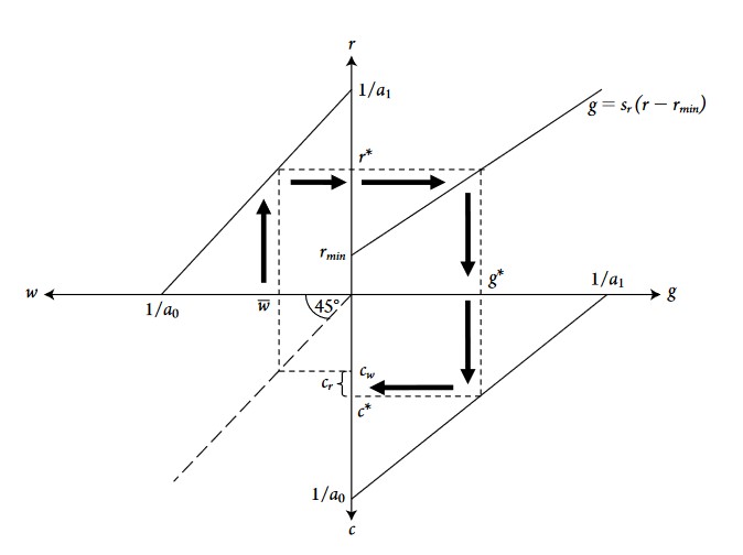
If the propsensity to save increases, the accumulation function curve becomes flatter (attention: in the graph above, the y and x axis are inverted on the right quadrant, where the accumulation function is drawn. So a rise in the slope implies a flattening of the curve). Since the real wage (or wage share) is exgenously given, it does not change. What changes are the growth (accumulation) rate and consumption: accumulation and growth increase because more profits are saved and invested into new capital. Consumption decreases because since capitalists increase their saving propensity, less of their profits are dedicated to personal consumption. Conversely, if the saving propensity decreases, accumulations and growth decrease and consumption increase. The real wage and profit rate remain unchanged.
\(\nearrow s_r \Rightarrow \nearrow I/K \Rightarrow \nearrow g, \searrow c\)
Closure 3 (natural rate of growth closure)
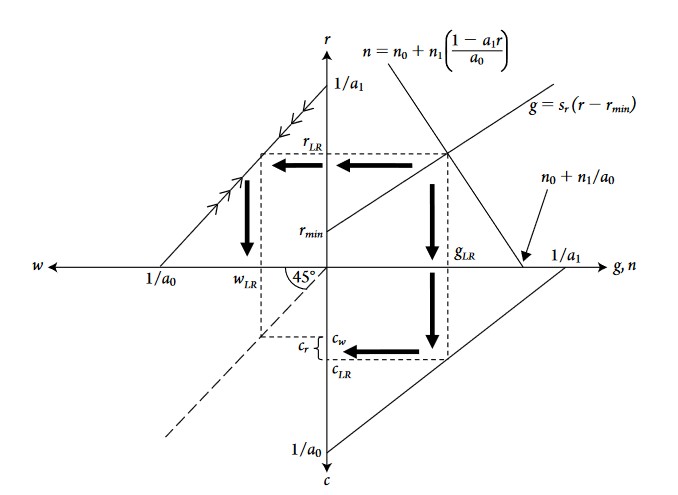
An increase in the propensity to save will again make the accumulation curve rotate down to the right (the slope increase). The direct short run effect is a rise in growth rate g. Then, this increase in growth rate makes labor demand increase faster than labor supply, resulting in a rise in the real wage. The rise in real wage decreases the profit rate and thus the growth rate decreases until the growth of labor demand and labor supply are equal. Whereas the growth rate g ends up at the same level or higher depends if labor supply is considered as endogenous or exogenous. If it is endogenous, the increase in labor supply after the increase in real wage will be faster and the new equilibrium growth rate will be higher than the original level. If labor supply is exogenous (a vertical curve in the upper-right candrant), the equilibrium growth rate cannot rise in the long run and will return at its original level.
Endogenous labor supply: \(\nearrow s_r \Rightarrow \nearrow \nearrow g, \Rightarrow \nearrow w, \searrow r \Rightarrow \nearrow n \Rightarrow \searrow g\),
but with final g > initial g. Note that under these conditions, both the growth rate and the real wage rise.
Exogenous labor supply: \(\nearrow s_r \Rightarrow \nearrow \nearrow g \Rightarrow \nearrow w, \searrow r \Rightarrow \searrow \searrow g\)
Closure 1 and 2
A rise in real wage or wage share would decrease the profit rate (recall the trade-off between wage and profit), which would decrease the growth rate (less is saved and invested since profits decrease). Consumption rises due to the increase in real wage/wage share
\(\nearrow \bar{w} \Rightarrow \searrow r \Rightarrow \searrow g \Rightarrow \nearrow c\)
A decrease in real wage or wage share would have the opposite effects.Closure 3 natural rate of growth
In this closure, a change in real wage or wage share would be the effect of an exognous change in population growth (and thus of labor supply). A rise in real wage would happen if there is a negative exogenous shock to population and labor supply (for instance a brutal epidemic like the black death, which decreased population a lot in the 14th century and made wages rise because of labor supply scarcity). The curve n = n0 + n1*w shifts to the left, real wages rise, profit rate decreases, growth rate decreases and concumption increases.
\(\nearrow n_0 \Rightarrow \nearrow w, \nearrow c \Rightarrow \searrow r \Rightarrow \searrow g\)
The manual presents four types of technological change:
Harrod-neutral: pure labor saving technological change
Labor productivity rises, but capital productivity remains unchanged
\(\nearrow Q = Y/L = 1/a_0\)
Hicks-neutral: factor-saving technological change
Both capital and labor productivity rise
\(\nearrow Q = Y/L = 1/a_0, \nearrow Y/K = 1/a_1\)
Marx-biased: labor saving, capital using
Labor productivity increases, but capital productivity decreases
Solow-neutral: pure capital saving technological change
Capital productivity rises, with labor productivity unchanged
All those patterns of technological change, with the exception of the marx-biased one, will improve the wage-profit trade-off, the curve of the latter shifting outward. Wage and profit as well as growth rise. Under the natural rate of growth closure (3) with exogenous labor supply, the long-run growth rate does not increase, however.
The FTRP is perhaps one of the most famous claim/theory of Marx. In Capital Volume III, Marx exposes this theory, which claims that technological change, by increasing labor productivity while decreasing capital productivity, will lead to a fall in the profit rate. The manual claims that Marx makes one important but often forgotten assumption: a constant rate of exploitation \(e = s/v\) with s the surplus value and v the value of labor power. Blecker and Setterfield argue that assuming a constant rate of exploitation is the same as assuming a constant wage share and profit share.
Recall that the profit share can be written as \(r = \pi / a_1\), if \(\pi\) the profit share is constant and marx-biased technological change happens, \(a_1\) will increase (\(a_1\) is the inverse of capital productivity \(a_1 = K/Y_k\)). and thus decrease profit rate \(r\). Thus, under the constant wage share closure, Marx-biased technological change does imply a fall in profit rate. However, it is unlikely that capitalists will let their profit rate fall without reacting and trying to suppress wages or slow down accumulation and growth, which would decrease labor demand, reduce workers bargaining power and thus lead to lower wages and to a recovery of the profit rate.
What about the third closure? Under this closure, the fall in profit rate does not happen, mainly because of the effect of the increase in labor supply resulting from the increase in real wage. If labor supply is considered as exogenous, the long run profit and growth rate cannot change: \(a_0\) falls more than real wage increase, and thus \(\pi = 1-wa_0\) increases. Thus, the FTRP is false under this closure, but another of Marx prediction is true: the relative immiseration of the proletariat, since the profit share increases (and wage share decreases).
Macroeconomic model simulation is a useful tool to understand and summarize the relationships between the endogenous and exogenous variables of a macroeconomic model. Here, I will simulate the effect of different shocks we have seen above on the given real wage and natural rate of growth closures. The R code I use to simulate the models is strongly inspired by the DIY Macroeconomic Simulation website, which explains how to run macro model simulations in R and Python with a lot of examples.
Before running the simulation and presenting the results, let’s first review and write down the model again. Under the exogenous real wage closure, we have 3 equations with 2 endogenous variables (I will here ignore consumption): \(g\) the growth rate and \(r\) the profit rate. The model has three parameters: the labour-output \(a0\) and capital-output ratio \(a1\), and the saving propensity out of profits \(s_r\).
\[ w = \bar{w} \] \[ r = \frac{1}{a_1} - \frac{a_0}{a_1}w \]
\[ g \equiv I/K \equiv S/K = s_rr \]
I will consider 4 scenarios. The first one is an increase the exogenous real wage \(\bar{w}\), the second one is an increase in the saving propensity out of profits \(s_r\), the third one a decrease in the labour-output ratio \(a_0\) (and thus an increase in labour productivity \(1/a_0 = Y/L\)) and the last one in the capital-output ratio (increase in capital productivity \(1/a_1 = Y/K\)).
Here is the code to run the simulation:
rm(list = ls()) # clean global environment

# five scenarios: baseline and 4 exogenous shocks
S = 5


# Create vectors for equilibrium values of the endogenous variables r and sr

r_eq = vector(length = S)
g_eq = vector(length = S)


# Create vector with parameter that will change
# We will consider exogenous shocks for each exogenous variable: w, sr, a0 and a1


# Scenario 1: increase in real wage w
w = vector(length=S)
w[] = 0.2 # (baseline value)
w[2] = 0.4

# Scenario 2: increase in saving propensity out of profits sr
sr = vector(length = S)
sr[] = 0.3
sr[3] = 0.4

# Scenario 3: increase in labour productivity 1/a0 (by decreasing a0)
a0 = vector(length = S)
a0[] = 1.5
a0[4] = 1.4

# Scenario 4: increase in capital productivity 1/a1 (by decreasing a1)
a1 = vector(length = S)
a1[] = 1.5
a1[5] = 1.4

# Setting endogenous variables at arbitrary positive value
g = r = 0.5

# Solve this system numerically through 1000 iterations based on the initialization

for (i in 1:S){
  for (iteration in 1:1000){
  r = (1/a1[i]) - ((a0[i]/a1)*w[i])
  g = sr[i]*r
  } # close iterations loop

#Save results for different parameterizations in vector
r_eq[i] = r
g_eq[i] = g

}
We can then compare the baseline values with the values of the different shocks. Here is the effect of the shocks on the equilibrium profit rate:
# Barplots for the effects of exogenous shocks on the profit rate

ggplot()+
  geom_col(aes(y = r_eq, x = c("Baseline", "Increase in w", "Increase in sr", "Increase in Y/L", "Increase in Y/K")))+
  labs(title = "Exogenously given real wage closure",
       subtitle = "Scenarios of 5 exogenous shocks",
       y = "Profit rate",
       x = "")+
  theme_minimal()+
  geom_hline(yintercept = r_eq[1])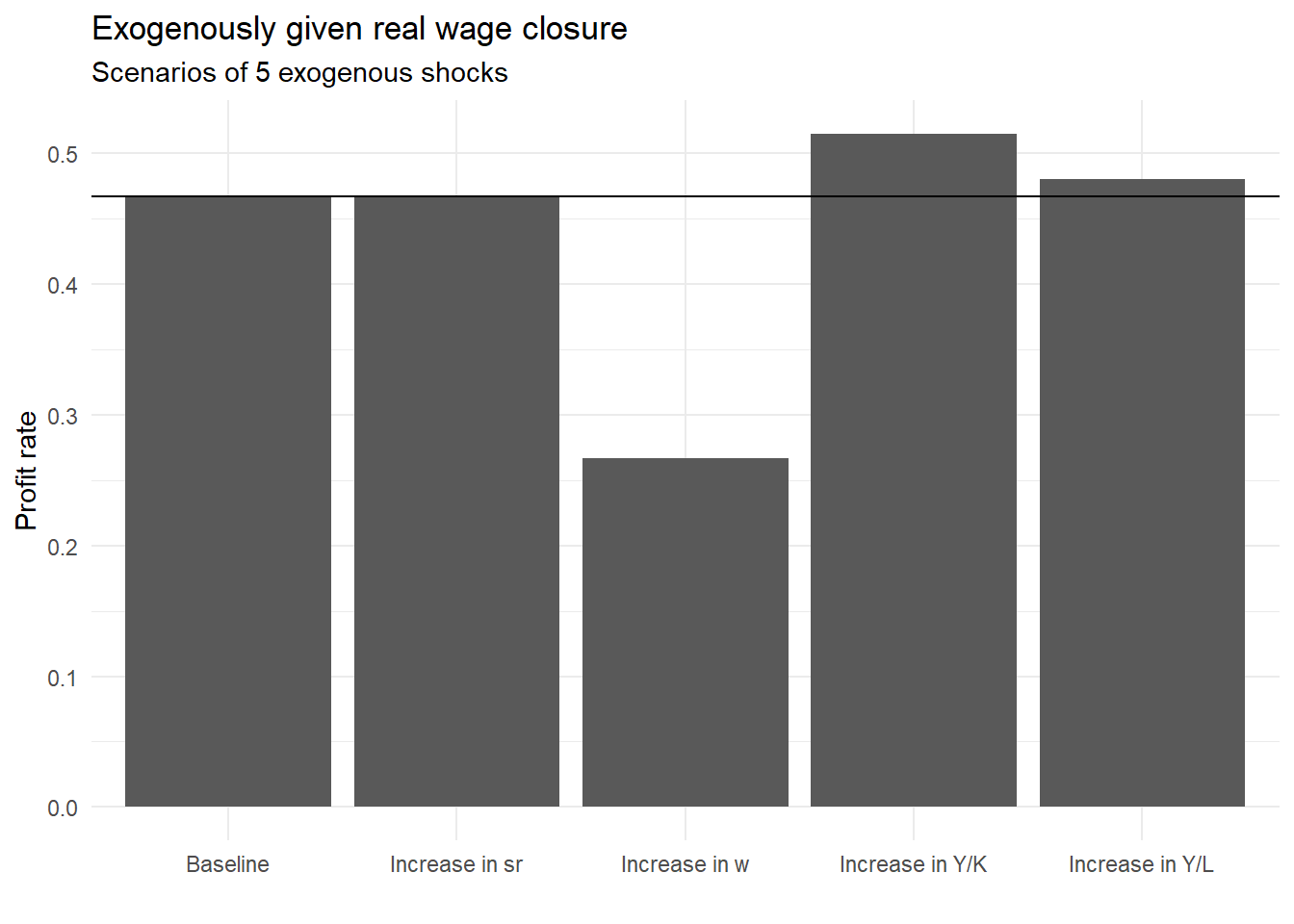
We can see that an increase in saving propensity out of profits has no effect on the profit rate. The reason is that, when \(a_0\) and \(a_1\) are assumed constant (no technological change), only variation in the real wage can affect the profit rate. An increase in real wage \(w\) decreases the profit rate, while increase in capital or labour productivity increases it.
What are the effects on the growth rate ?
# Barplots for the effects of exogenous shocks on the capital accumulation (growth) rate g

ggplot()+
  geom_col(aes(y = g_eq, x = c("Baseline", "Increase in w", "Increase in sr", "Increase in Y/L", "Increase in Y/K")))+
  labs(title = "Exogenously given real wage closure",
       subtitle = "Scenarios of 5 exogenous shocks",
       y = "Growth rate g",
       x = "")+
  theme_minimal()+
  geom_hline(yintercept = g_eq[1])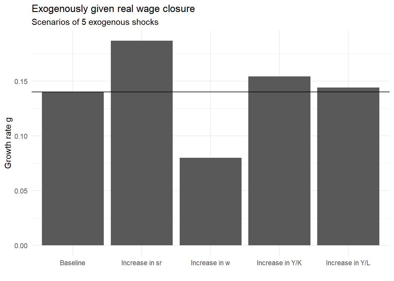
An increase in saving propensity increases the equilibrium rate of growth, because more profits are saved and thus invested in the economy. An increase in real wage decreases the profit rate, which decreases the amount of savings out of profit and thus investment and growth. Technological change, whether through capital or labour productivity increase, increases the equilibrium growth rate.
In the natural rate of growth closure, the real wage is not exogenous but adjusts to balance labour supply \(n\) and labour demand, assumed to be closely proportional to the rate of growth \(g\). Labour supply is assumed to be a positive linear function of the real wage: \(n = n_0 + n_1w\). The equilibrium condition is the balance between labour supply and demand: \(g = n\). We have thus four endogenous variables: \(w\), \(r\), \(g\), and \(n\); and five parameters/exogenous variables: \(a_0\), \(a_1\), \(s_r\), \(n_0\) and \(n_1\). The model’s equations are:
\[ w = \frac{1}{a_0}-\frac{a_1}{a_0}r\] \[ r = \frac{1}{a_1} - \frac{a_0}{a_1}w \] \[ g = s_rr \] \[ n = n_0 + n_1w, \qquad n_0,n_1>0 \]
I will consider four scenarios: an increase in saving propensity out of profit \(s_r\), a decrease in population growth independent from a decrease in real wage \(n_0\), a rise in labour and capital productivity (\(1/a_0\), \(1/a_1\)).
Here is the code to simulate these scenarios:
# simulate exogenous shocks for the natural rate of growth closure

rm(list = ls())

# Three scenarios: baseline, increase in n0, and sr
S = 5

# Set parameters values

n1 = 0.1


# Create vectors for equilibrium values

r_star = vector(length = S)
g_star = vector(length = S)
n_star = vector(length = S)
w_star = vector(length = S)

#Create vector with parameter that will change
sr = vector(length = S)
sr[] = 0.5
sr[2] = 0.8

n0 = vector(length = S)
n0[] = 0.1
n0[3] = 0.08

#
a0 = vector(length = S)
a0[] = 3
a0[4] = 2

#
a1 = vector(length = S)
a1[] = 3
a1[5] = 2

# Initialise endogenous variables at arbitrary positive value
w = r = g = n = 1

# Solve this system numerically through 1000 iterations based on the initialisation

for (i in 1:S){
  for (iteration in 1:1000){

    w = (1-a1[i]*(r))/a0[i]
    r = (n0[i] + n1*w)/sr[i]
    g = sr[i]*r
    n = n0[i] + n1*w
  } # close iterations loop

#Save results for different parameterisations in vector

  w_star[i] = w
  r_star[i] = r
  g_star[i] = g
  n_star[i] = n

}
Let’s first have a look to the effects on the growth rate of capital accumulation.
ggplot()+
  geom_col(aes(y = g_star, x = c("Baseline", "Increase in sr", "Decrease in n0", "Increase in 1/a0", "Increase in 1/a1")))+
  labs(title = "Natural Rate of Growth Closure",
       subtitle = "Effect of exogenous shocks on the growth rate g",
       y = "g", x = "")+
  theme_minimal()+
  geom_hline(yintercept = g_star[1])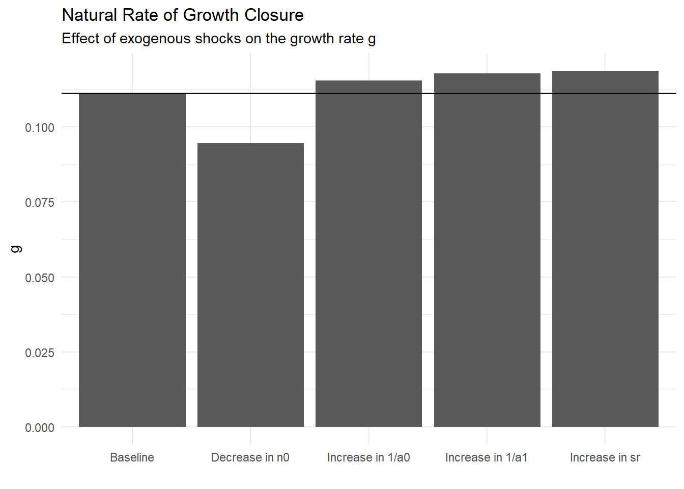
A decrease in \(n_0\) (due to, for instance, lower birth rate, reduced immigration flows or restrictions on child labour) has a negative impact on the equilibrium growth rate. Labour supply decreases, making labour more scarce and thus more expensive for capitalists, who need to offer higher real wage, which reduces the profit rate and thus savings, investment and accumulation. An increase in saving propensity, as in the exogenous real wage closure, increases the growth rate (more savings and thus more investment and growth). Labour and capital productivity both increase the growth rate.
The effects on the profit rate are:
ggplot()+
  geom_col(aes(y = r_star, x = c("Baseline", "Increase in sr", "Decrease in n0", "Increase in 1/a0", "Increase in 1/a1")))+
  labs(title = "Natural Rate of Growth Closure",
       subtitle = "Effect of exogenous shocks on the profit rate r",
       y = "r", x = "")+
  theme_minimal()+
  geom_hline(yintercept = r_star[1])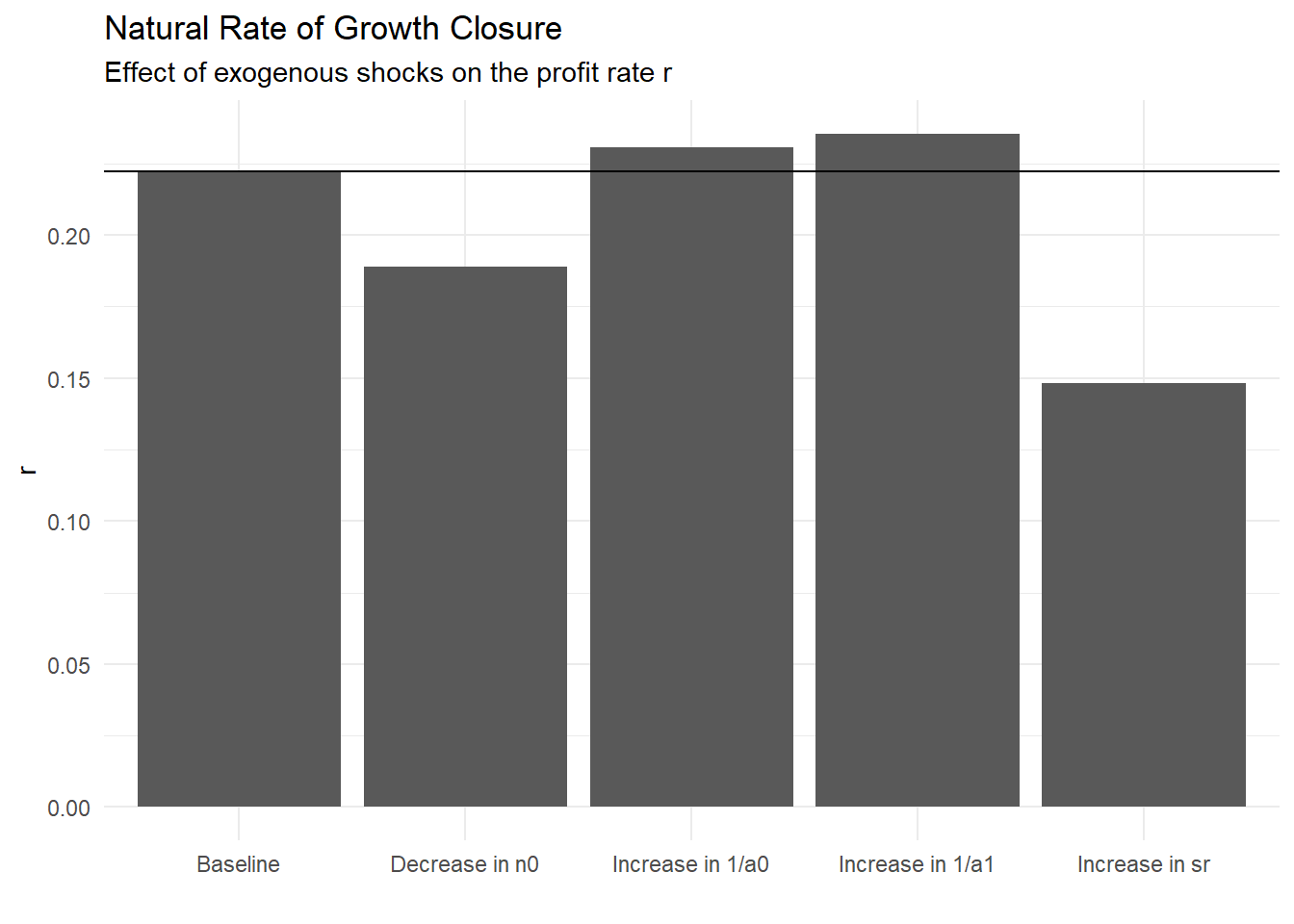
It is interesting to underline the negative effect of an increase in saving propensity on the profit rate. Why is it the case ? When saving rate rises, a higher share for each unit of profit is saved and thus less profits are required to finance the same amount of investment and accumulation. An increase in \(s_r\) increases savings, investment and growth, which increase labour demand faster than labour supply. Real wage thus increases until labour demand and supply are balanced. As real wage increases, the profit rate declines. Note that, if \(n_1 = 0\) and thus labour supply growth is exogenous and independent from real wage, the equilibrium profit rate would also fall, but the equilibrium growth rate remains unchanged because labour supply growth would not have increases after the increase in real wage. An exogenous decrease in labour supply growth reduces the profit rate because labour supply growth would be lower than supply and thus real wage would increase.
Finally, let’s have a look at the effects on the real wage:
ggplot()+
  geom_col(aes(y = w_star, x = c("Baseline", "Increase in sr", "Decrease in n0", "Increase in 1/a0", "Increase in 1/a1")))+
  labs(title = "Natural Rate of Growth Closure",
       subtitle = "Effect of exogenous shocks on the real wage w",
       y = "w", x = "")+
  theme_minimal()+
  geom_hline(yintercept = w_star[1])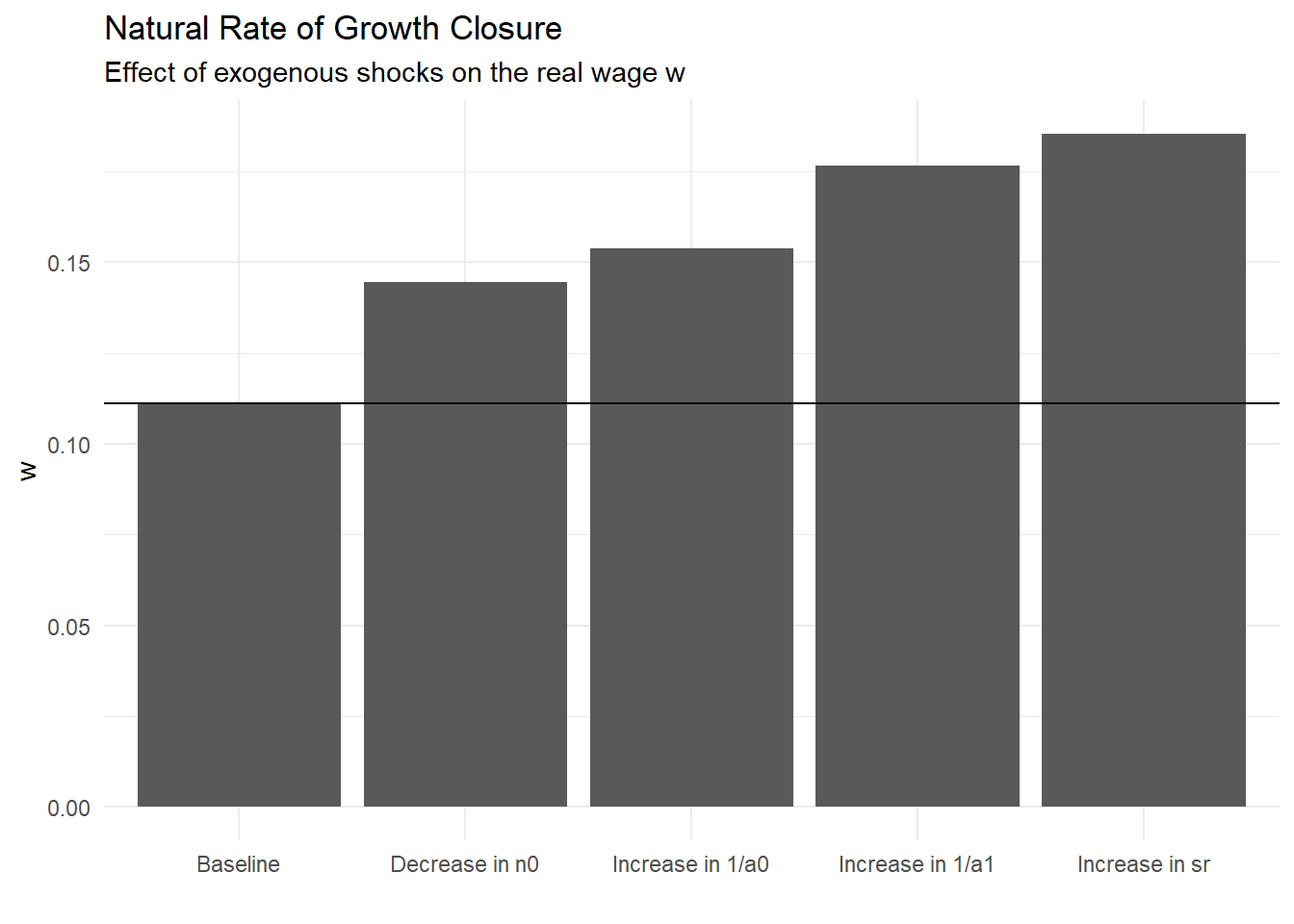
It is important to stress that, for the first time, we see that real wage and the growth rate both increase after a rise in saving propensity. An exogenous decrease in labour supply growth also increase the equilibrium real wage, as labour demand would grow faster than labour supply until real wage rises to balance labour demand and supply.
The classical-marxian models presented above are concerned about long-term growth. Marx is however also known to have developed an interpretation of business cycles or cyclical growth in the 25th chapter of Capital Volume I. In that chapter, Marx described a dynamic relationship between the real wage and the profit share. In a period of rapid growth, the real wage increase (because of higher bargaining power of workers due to higher employment rate) leads ultimately to a lower profit share. Because the profit rate is declining, capitalists invest less and thus cause a recession. Accumulation slows and, as unemployment rises, workers loose bargaining power and their wage share thus falls (leading to a higher profit share). When the wage share has fallen enough so that capitalists are willing to invest more in the economy, the economic downturn leaves place to an expansion and the cycle repeats.
The economist Richard Goodwyn (1913 - 1996) was the first to elaborate a mathematical model based on Marx’s business cycle. His model is now known in the literature as the “Goodwyn cycle”.
This model consists of two differential equations for the employment growth rate \(\hat{e}\) and the growth rate of the wage share \(\hat{psi}\):
\[ \hat{\psi} = - (q + y) + ce \\ \hat{e} = \frac{1 - \psi}{a_1} - (n + q) \]
With \((n + q)\) the natural rate of growth (the maximum rate of growth an economy can achieve, which is the sum of employment growth rate \(n\) and productivity growth rate \(q\)); \(c\) and \(y\) some positive constants.
The model assumes that all profits are saved and invested; that the rate of capital accumulation is equal to the profit rate, that \(a_1\) is constant (no productivity growth) and that labour supply growth \(n\) is exogenous.
The model is thus a system of two linear dynamical equations. The analysis of a model of two differential equations is different from the previous models and involve the following steps (Sayama 2015, p.126-127):
Find the equilibrium points by setting our (differential) dependent variables equal to zero. This gives the nullcline curves at which the rate of growth of our dependent variables are equal to zero.
Calculate the Jacobian matrix of the system and its eigenvalues.
The real part of the dominant eigenvalue \(\lambda_d\) determines the stability of the whole system:
Let’s apply this procedure to our Goodwyn model
\[e^* = \frac{q + y}{c}\]
and for \(\hat{e} = 0\), we have:
\[\psi^* = 1 - a_1(n+q)\]
If one plots the level of the wage share \(\psi\) on the y axis against the level of employment \(e\) on the x axis, these two nullclines gives us one vertical line at \(\frac{q + y}{c}\) and one horizontal line at \(1 - a_1(n+q)\).
Even without computing the Jacobian matrix and its eigenvalues, one can have a broad idea of how the system behaves in the four regions divided by the nullcline. To do so, we can simply solve the system for some values in the four regions. For instance, if we want to see how the rate of growth of the wage share and employment rate move in the right-upper region, we can set two values for \(e\) and \(\psi\) which are above the two nullcline. For example, if \(e = 2(\frac{q+y}{c})\) and \(\psi = 2(1-a_1(n+q)\), we get:
\[ \hat{\psi} = q + y \\ \hat{e} = (n+q) - \frac{1}{a_1} \]
It is clear that \(\hat{\psi} = q + y\) is necessarily positive, because both q and y are positive constants. Whereas the sign of \(\hat{e}\) is less clear, it needs to be negative because the natural rate of growth, which is usually moderate, is subtracted from the level of productivity which takes larger values than the natural growth rate.
At these two points, the rate of growth of the wage share is increasing and the rate of growth of employment is decreasing. We are at the point in the model in which there is a recession due to increase in the wage share which reduces profitability.
Doing that for the four region, we can then obtain the following graph.
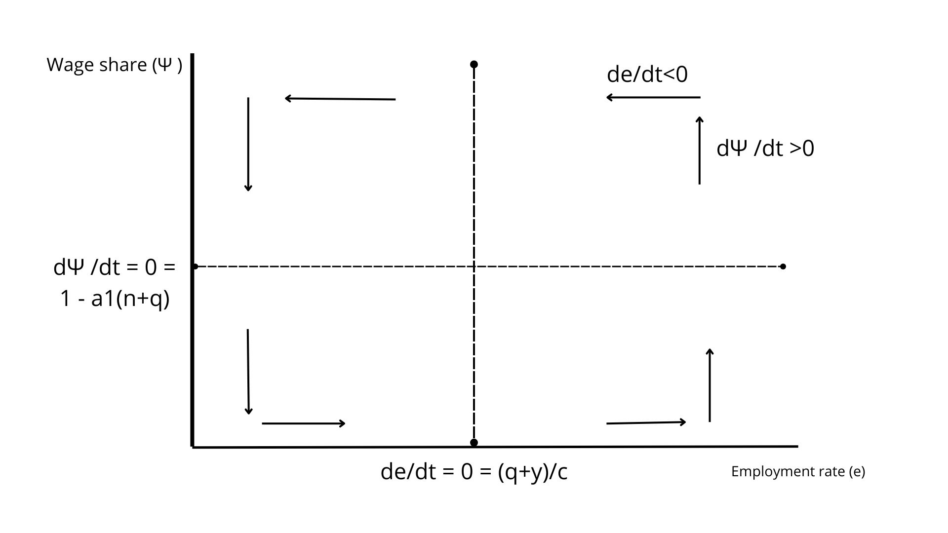
By doing this, we can see how the wage share and employment rate grow in the four regions. However, we still don’t know the asymptotic behavior of the system (that is, the behavior of the system in the long run). to explore whether the system reaches an equilibrium point or diverges from the latter, or circulates perpetually around it, we need to compute the Jacobian matrix and then its eigenvalues.
The Jacobian matrix is a matrix composed of the partial derivative of the two equation constituting the system (note that for this system, the Jacobian matrix is equivalent to the coefficient matrix). Since the two equations do not have their own level values as dependent variables, we need only to compute the derivative of \(\hat{\psi}\) with respect to \(e\):
\[ \frac{d\hat{\psi}}{de} = c \]
and the derivative of \(\hat{e}\) with respect to \(\hat{\psi}\):
\[ \frac{d\hat{e}}{d\psi} = -\frac{1}{a_1} \]
The Jacobian is thus:
\[ J = \begin{bmatrix} 0 & c\\ -1/a_1 & 0 \end{bmatrix} \]
Computing the eigenvalues, we arrive at:
\[ \det(J - \lambda I) = \lambda^2 + \frac{c}{a_1} = 0 \\ \lambda = \pm i \sqrt{\frac{c}{a_1}} \]
With \(\lambda\) the eigenvalues being imaginary numbers with no real part, this means that the system is neutral stable (also said Lyapunov stable). That means that we have a cycle which perpetually circles around the equilibrium point.
We can check this by running a simulation. The code below shows how to do this in R. I use the Euler forward method, which is not ideal for a system of differential equations, but does the work with enough time period and a low enough step size.
t = 50000

psi = rep(NA, t)
e = rep(NA, t)

psi[1] = e[1] = 0

#set parameters values
q = 0.01
a1 = 1.17
n = 0.001
c = 1
y = 0.80

delta_t = 0.001

for (i in 2:t) {

  psi[i] = psi[i-1] + delta_t * (-(q + y) + c*e[i-1])
  e[i] = e[i-1] + delta_t * (((1-psi[i-1])/a1) - (n + q))

}


psi_eq = 1 - a1*(n + q)

e_eq = (q + y)/c

results = tibble(psi, e, t = 1:t)