In economics and social sciences in general, factor analysis is a very useful set of methods used to analyze data for a wide variety of topics. The most well-known method is principal component analysis (PCA), which allows to reduce a set of variables into a few “principal components” which are linear combinations of the datasets’ variables. The components are ordered according to the percentage of variance captured by it and components are orthogonal (not correlated) with each other. PCA applies only to quantitative variables, but there are many options to include qualitative and ordinal variables: multiple correspondence analysis (MCA) which applies to qualitative variables only, and mixed methods which applies to both qualitative and quantitative variables. Factor analysis is also useful to run cluster analysis. Once the principal components are estimated, hierarchical cluster (HC) can be conducted to groups the observations into clusters.
However, what happens when our variables correspond to different group ? Running a PCA directly would ignore this grouping and thus loose a lot of information. To give an example I am studying, the literature on comparative capitalism often uses clustering through PCA and MCA to identify empirically the varieties of socio-economic models which exist across countries. One of the main ideas of comparative capitalism is that social, political and economic institutions come with different forms, hierarchy as well as complementarities within countries, leading thus to different forms of capitalism between them, that we can clusterize. This is what has been done by, for instance, Amable (2003) who identified five types of capitalism by the analysis of five institutional domains: the wage-labour nexus; the financial system; the education system; product-market competition; the welfare state & social protection system. Cahen-Fourot (2020) offers a similar typology, but with slighlty different institutional domains (which he calls “institutional forms” because they are taken from Régulation Theory): the monetary regime; the wage-labour nexus; the form of competition; the form of the state and the insertion into the international regime. What is interesting in Cahen-Fourot (2020) is that he includes an additional institutional form: the social relations to the environment.
To identify and cluster different types of capitalism, this literature uses a combination of PCA and MCA through the following steps:
Run a PCA for each institutional domain separately
Cluster the countries on this institutional domain using HC on the PCA and attribute each country to their cluster
Run a MCA on the cluster classification
Despite the fact that this approach is acceptable, it can be very time consuming especially when the steps 1 and 2 above must be repeated a lot (in the example above, 5 or 6 times). There exists another principal component method which allows to do that in a much simpler way: multiple factor analysis. Using this method would allow to run a single principal components dimension reduction while taking into account the fact that the data are grouped into categories (in that case the institutional forms) and thus avoiding to run a separate analysis for each one of them. In very simple terms, MFA can be considered as a weighted PCA in which each variable is divided by the square root of the first eigenvalue of the group it belongs to. By doing so, the group structure is preserved while running the analysis over all the variables.
The present post will not explain further details on MFA, but will focus on its practical implementation and visualization in R using the FactoMineR and FactoShiny packages. There are many resources online to learn all technical details about MFA, as this series of youtube tutorials done by François Husson. this post is also very useful.
How to run MFA in R
To show of to run MFA in R, I will use the data compiled by Cahen-Fourot (2020) to analyze the diversity of capitalisms in 2015. This data contain 76 variables covering 37 countries.
library(readr)data <-read_csv("data_full_CF2020.csv") %>%column_to_rownames(var ="Country") %>%# important to have countries as rownames or the MFA will consider them as qualitative indicator variableselect(-c(MatfootGDP, CO2footGDP, EnerfootGDP)) # remove three variables which are present in the dataset but will not be usedhead(data) %>%gt()
SCP
GIN
DCB
GOV
PCT
CCR
ABC
ABP
BSS
LPS
CSR
LBR
ATX
BEN
FDI
TRF
TFS
TRD
Telec_struc
Elec_struc
Gas_struc
Post_struc
Rail_struc
Hstat
LernerIndex
StateControl
Taxes
HealthGDP
EducGDP
MilitaryGDP
Finalcons
HealthGOV
EducGOV
MilitaryGOV
Int_rate
Inf_rate
Fin_reg
LLR
FinOpen
Liq
PrimAgri
PrimIndus
SecManuf
SecConst
Ter_Serv
Ter_FIRE
Tradeglobfacto
Finglobfacto
Tradeglobjure
Finglobjure
Socglobfacto
Socglobjure
Polglobfacto
Polglobjure
IUCN
GreenP
EnvConflicts
ClassGHG
EnvReg
EnvTreaties
EnfEnvReg
EnerGDP
GHGGdp
MatGDP
MatEmb
EnerEmb
CO2Emb
Wshare
DistProf
Labprotec
CollBarg
Unions
Unemp
IncomeIneq
WorkingHours
Gender
2.85
2.17
1.03
5.63
0.84
1.08
0.8
0.8
1.15
4
0.55
1.47
1.43
2.75
0.77
0
0.00
0.00
1.60
0.0
0.00
3
3.0
0.31
0.17
1.94
22.1
6.1
5.32
1.96
18.1
16.65
14.08
5.22
2.26
1.51
1389
0.54
0.94
1874
0.02
0.10
0.07
0.09
0.50
0.22
239
785
839
678
868
800
908
911
1.28
0.213
0.7
5.5
5.7
24
5.7
0.100
408
0.70
-131.2
-9.1
1.9
58.8
15.0
1.9
50.6
15.0
6.1
0.3
34
13.0
3.00
2.78
1.03
2.25
0.37
1.78
1.8
0.2
4.04
2
0.05
0.20
0.00
2.47
0.63
0
0.35
1.40
1.36
0.0
1.50
2
0.0
0.71
0.55
1.67
26.8
7.8
5.45
0.71
19.9
15.10
10.70
1.37
-0.02
0.90
1654
2.65
1.00
2971
0.01
0.03
0.18
0.06
0.56
0.15
699
907
911
737
871
864
939
973
0.59
0.115
0.7
3.4
6.2
25
6.1
0.079
190
0.42
56.9
8.4
25.9
63.7
16.8
2.4
98.0
27.4
5.7
0.3
35
17.0
2.60
2.59
1.16
3.00
1.17
2.92
2.2
1.0
4.40
2
0.94
1.50
0.00
2.52
0.24
0
0.50
0.00
1.51
1.5
0.00
2
3.0
0.68
0.17
2.19
24.7
8.6
6.55
0.92
23.9
16.02
12.17
1.71
-0.02
0.56
1869
2.88
1.00
2081
0.01
0.03
0.13
0.06
0.63
0.15
932
936
880
818
826
899
926
990
1.16
0.846
0.4
3.6
5.5
26
5.2
0.104
231
0.29
53.7
-81.4
-1.4
66.8
15.9
3.0
96.0
54.2
8.5
0.3
35
4.7
2.64
1.77
2.29
4.00
2.53
2.17
3.6
2.0
3.43
6
1.57
2.07
0.00
3.44
0.61
4
0.80
3.55
1.93
0.0
6.00
3
6.0
0.74
0.01
2.51
12.8
3.8
6.24
1.36
19.7
7.66
16.25
3.57
14.25
9.03
1636
20.40
0.17
6135
0.05
0.07
0.14
0.06
0.53
0.15
191
501
479
285
453
766
955
676
0.10
0.017
0.5
14.4
4.7
24
3.7
0.125
439
1.47
-13.8
4.6
12.1
50.3
21.1
1.7
70.5
19.5
8.4
0.5
39
16.0
2.60
1.92
0.59
3.75
1.95
1.30
0.0
0.2
3.75
2
0.57
0.69
0.65
2.95
1.04
0
1.84
1.17
1.57
3.0
0.00
2
1.5
0.81
0.39
1.92
12.3
7.7
5.27
1.16
20.9
19.07
12.22
2.87
0.82
1.13
142
4.69
1.00
3762
0.02
0.10
0.11
0.07
0.52
0.19
365
841
859
748
888
842
933
937
0.62
0.253
0.7
6.8
5.0
19
5.0
0.151
400
0.58
13.7
3.8
3.5
63.4
16.0
1.5
30.6
28.6
6.9
0.3
35
18.6
2.47
1.79
0.96
3.75
2.39
1.50
1.2
0.8
1.37
6
1.50
0.47
0.00
3.11
0.34
0
0.10
1.26
1.30
0.0
0.75
1
4.5
0.81
0.40
2.10
17.5
4.9
4.87
1.91
13.2
19.58
19.59
7.62
4.94
4.35
1262
0.52
0.70
1929
0.04
0.14
0.11
0.08
0.43
0.05
382
769
772
643
581
819
853
913
0.17
0.039
2.8
8.5
4.7
22
4.7
0.136
433
2.77
-188.5
5.5
8.2
44.8
25.3
1.8
17.6
17.9
6.5
0.5
42
21.1
The first 25 variables concern the form of competition. In Regulation Theory, the form of competition (akin to product market competition in the varieties of capitalism framework) captures the nature and degree of competition in the socio-economic model. Institutions which constitute this form are for instance administrative burdens to for corporation (ABC), sole proprietor firms (ABP), entry barriers, price controls (PCT), or the degree of competition (measured here by the Lerner index).
The next 9 variables are for the wage-labour nexus, which comprises all institutions regulating employment relationships, wage setting, work organization and social protection.
The monetary regime, defined as all the institutions regulating money, credit and finance, is summarized by 6 variables (interbank 3-months interest rate, inflation rate…) while 14 variables describe the insertion into the international regime such as the importance of agriculture (PrimAgri), extractive industries (PrimIndus), manufacture (SecManuf) and the so-called globalization index from the KOF economic institute. Finally, the social relations to the environment is captured by the remaining 9 variables such as environmental regulation stringency (EnvReg), GDP intensity in greenhouse gas (GHGGDP).
To run MFA in R, one just needs to load the FactoMineR package and use its MFA() function. The only complication of this function is the group argument it needs to be a vector of numbers which describe how the variables are grouped. It works as follows:
# create a vector with the name of the groups (ie the 6 institutional forms)group_name <-c("Competition", "State","Money", "International regime", "Environment","Wage-labour nexus") MFA_CF2020 <-MFA(data, group =c(25, 9, 6, 14, 13, 9), type =rep("s", 6), ncp =5, # manumber of principal components to keep name.group = group_name, graph =FALSE)
group = c(25, 9, 6, 14, 13, 9) tells the function that the first 25 variables are the first group, the second group then contains the following 9, then the third the following 6 etc. One can also give the groups name with the group_name argument. type = rep("s", 6) tells the nature of the variables for each group. “s” is for quantitative variables and thus we have to repeat this string 6 time for the six groups (hence the rep function).
Apart from the group argument, we can appreciate of simple it is to implement MFA in R, while conducting separate analyses using 6 PCA and MCA six time would have required much more time and code. The only drawback of the MFA() function is that it requires the variables to be ordered by groups in the dataframe.
Exploring separate PCA
The MFA function returns an list with two main elements:
separate.analyses: those are PCA analyses for each group. We have thus 6 separate PCA analyses for each institutional forms and we can analyse, visualize and perform cluster analysis on each of them if we are interested.
global.analysis which is the global PCA with the variables weighted accordingly to their group.
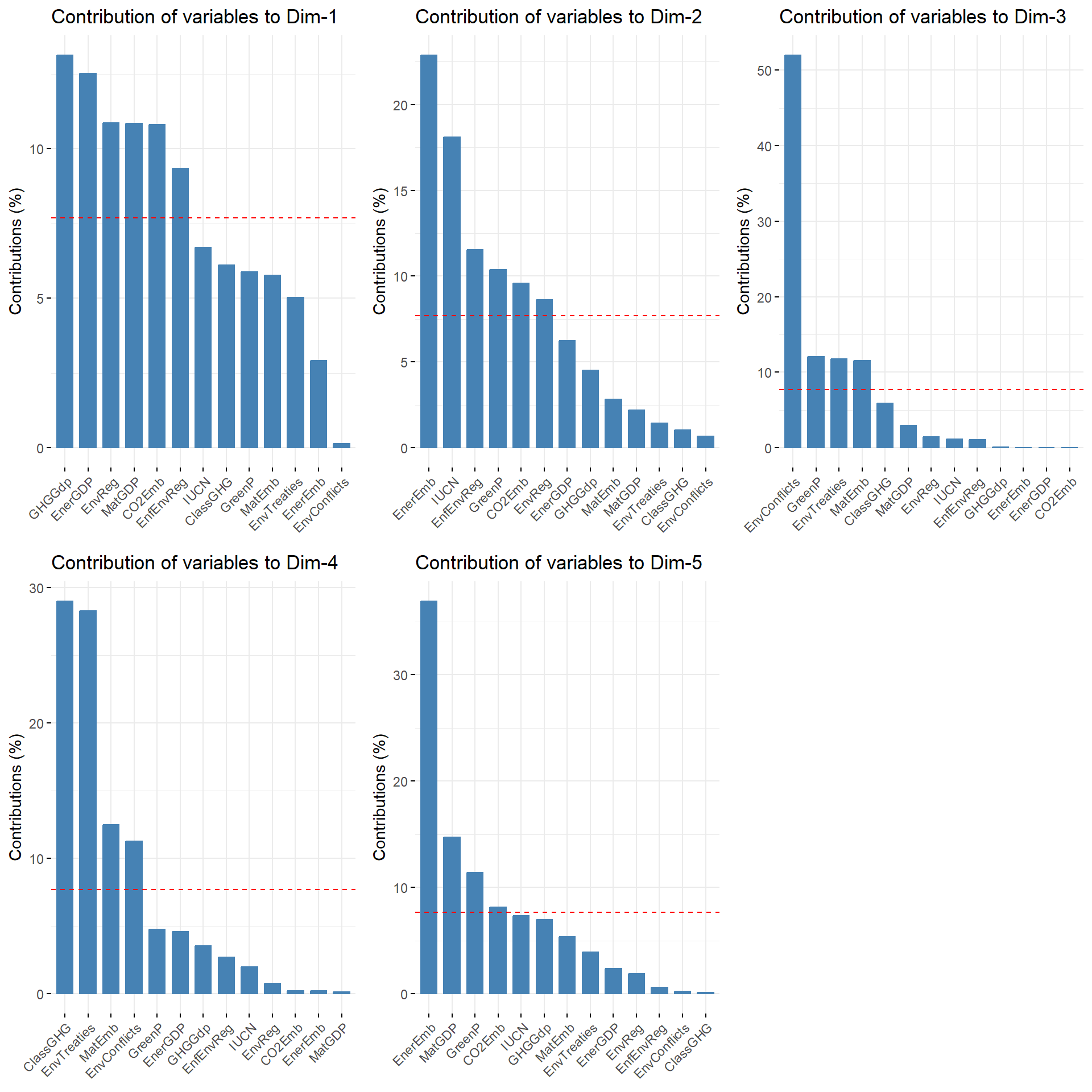
For instance, let’s have a look the to the social relations to the environment. It is common practice in factor analysis to first have a look to the contribution of the dataframe’s variables to the principal components. There are two graphs which help to visualize this: a barplot plotting the variables’ eigenvalues and the circular plot. It is very straightforward to produce such a barplot in R thanks to the factoextra package and its fviz_contrib function. Below, I show how to generate these graphs for the first 5 principal components, store them into a list and plot them together with the ggarange function from ggpubr package:
library(ggpubr)barplots_contrib_env <-1:5|># we want 5 plots for the first 5 PC, so I provide a vector which will integrated in the map function through axes = .x argumentmap(~fviz_contrib(MFA_CF2020$separate.analyses$Environment, choice ="var", axes = .x))ggarrange(plotlist = barplots_contrib_env)
We have now an overview to how the first five PCs are structured. The first PC is highly correlated with variables such as GDP intensity in GHG (GHGGdp) and energy (EnerGDP), as well as environmental regulation stringency (EnvReg). The second PC is correlated with embodied energy in net imports relatively to energy consumption (EnerEmb) and organizations member of IUCN per millions inhabitants. The variable capturing environmental conflict contribute more than 50% to the third PC.
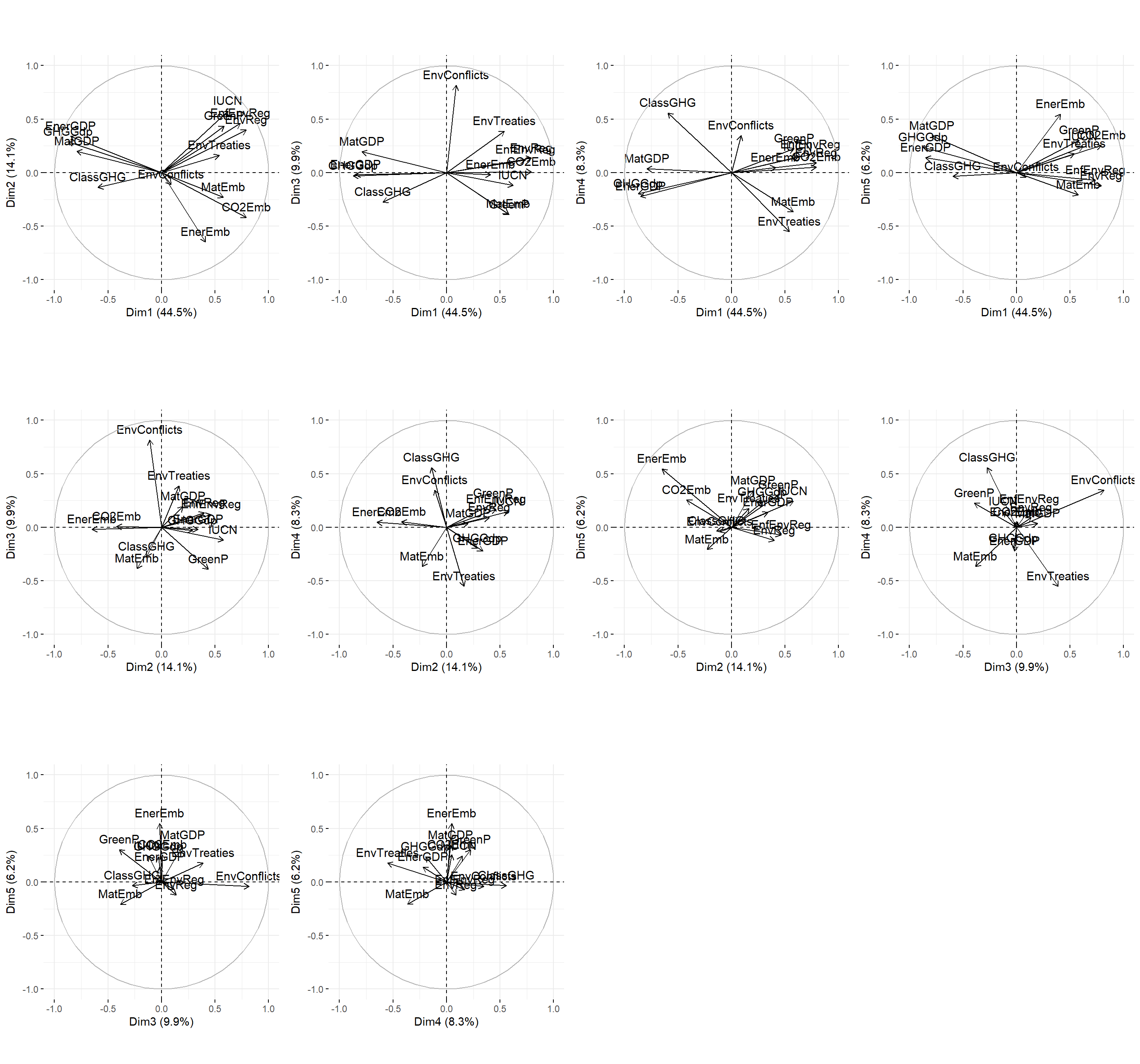
However, the barplots do not tell us to whether the variables which contribute the most to the PCs are correlated negatively or positively to the latter. To see that, circular plots are a good visualization. Here, the code is slighlty more complex because we need to provide a five elements list in which there are the combinations of the PCs represented in the circular plot:
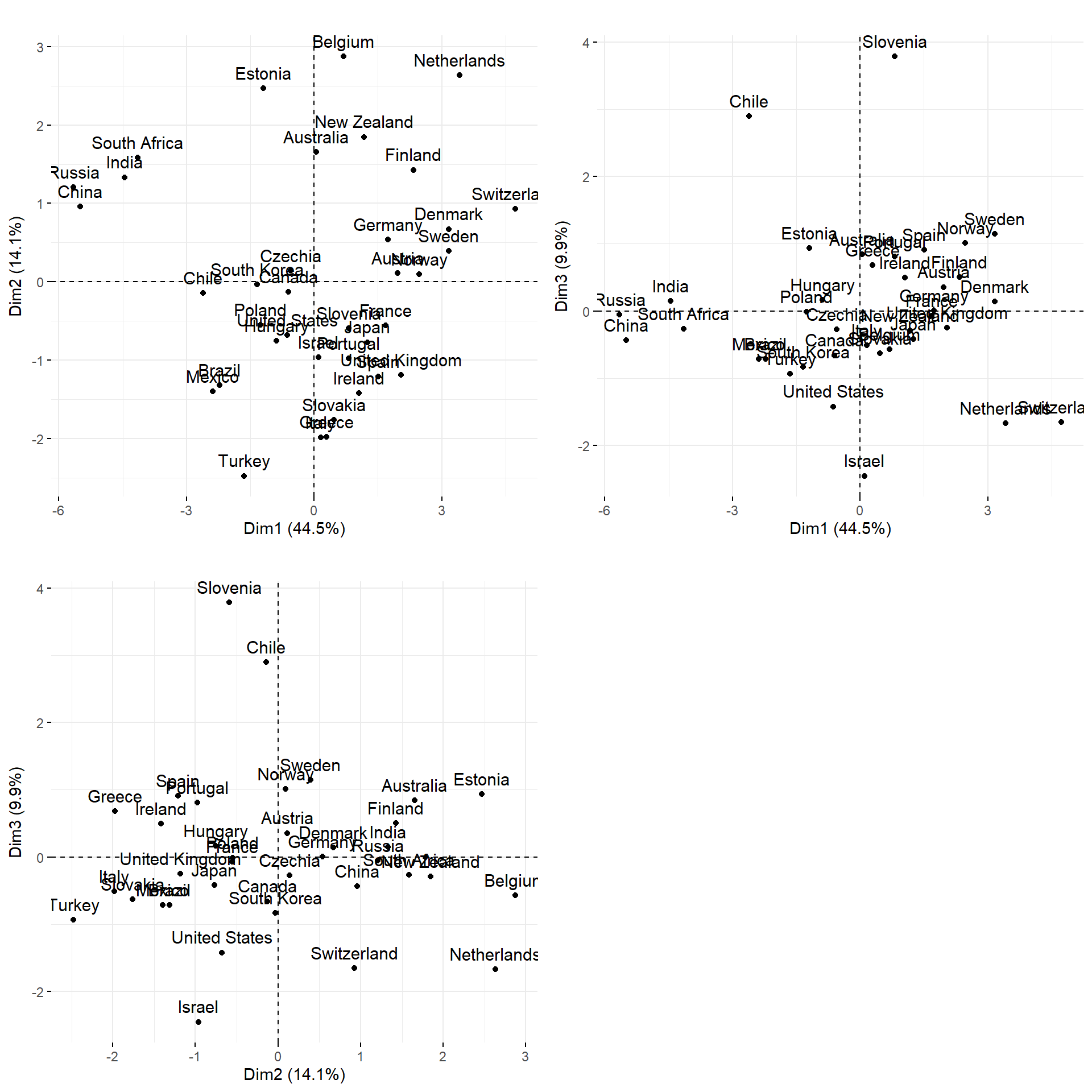
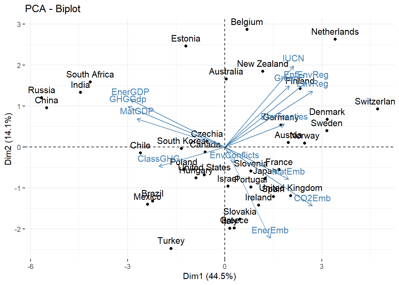
From the graphs above, one can make the following observations regarding the position of countries on the two dimensions. On the upper right quadrant, we have countries which are characterized by (relatively) a lot of climate activism (measured by IUCN and GreenP), environmental regulations and enforcement, but are also characterized by some important degree of CO2 offshoring (EnerEmb and CO2Emb measure energy and CO2 in net imports, they measure the degree of offshoring of GHG emissions). On the upper left quadrant, we have countries such as China and India with high domestic GHG emissions (EnerGDP, GHGGDP…), high carbon inequalities, low offshoring and climate activism. On the lower right quadrant, we have countries such as France and the UK which have relatively lower domestic GHG emissions but with high offshoring and low activism.
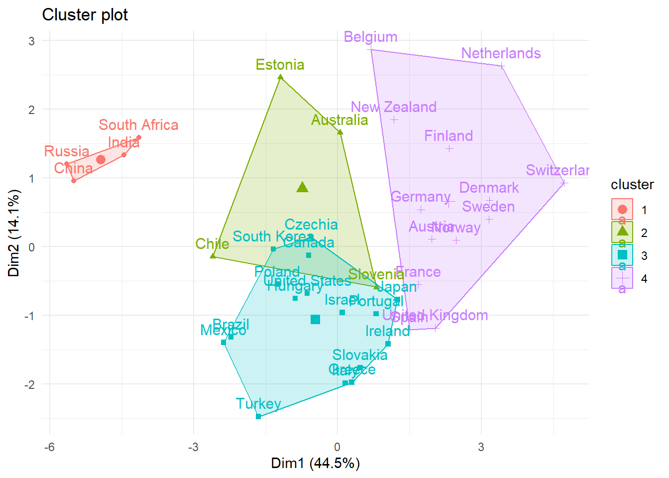
Applying hierachical clustering is also very easy through the HCPC() function. Note that it is not possible to run this function in quarto since the function asks to cut the dendogram tree to determine the number of clusters. I thus ran the code first in a R script to get the number of clusters which is four:
The clusterization confirms the obervations we made above: we have a group of domestic polluters (cluster 1), low offshoring (which makes sense since they export their domestic pollution to rich countries of cluster 4 and 3) and lower activism. Cluster 3 gathers countries with high carbon inequalities and relatively higher carbon emissions (lower than cluster one but higher than cluster 4) and low activism. Cluster 4 is mostly composed of rich countries with high degree of offshoring, activism, lower inequality and GHG emissions.
Exploring global PCA
Let’s now have a look to the global weighted PCA. Let’s start with the contribution of the variables on the first two dimensions. Since there are a lot of variables, it is useful to make an interative plot with the ggplotly function from the plotly package so that we can zoom on the graph:
We can see that the first principal component is highly positively correlated with the degree of labour protection and BSS (entry barriers in professional services, freight transport services and retail distribution) while the second is highly correlated with the variables measuring the degree of domestic pollution and negatively correlated with globalization indicators, collective bargaining, the wage share and climate activisms (among other…).
Amable, Bruno. 2003. The Diversity of Modern Capitalism. OUP Oxford.
Cahen-Fourot, Louison. 2020. “Contemporary Capitalisms and Their Social Relation to the Environment.”Ecological Economics 172 (June): 106634. https://doi.org/10.1016/j.ecolecon.2020.106634.